Data exploration of a climate database using SQLite and SQLAlchemy
Project background
This project used an SQLite database to extract data on weather measurements at weather stations in Hawaii. The data was first explored to find any interesting insights into the weather patterns, using SQLAlchemy to query the database. Then, an API app was created to query the database and return JSON results when a user selects certain endpoint routes.
Exploratory Climate Analysis
Precipitation Analysis
Weather Station Analysis
Preparation for the Analysis
- As a first step, we need to import Matplotlib to graph the results of the analysis. For this project we we'll use the "fivethirtyeight" style for Matplotlib graphs.
Import dependencies for graphs:
%matplotlib inline
from matplotlib import style
style.use('fivethirtyeight')
import matplotlib.pyplot as plt- Next, add NumPy and Pandas:
import numpy as np
import pandas as pd- Import datetime dependencies:
import datetime as dt- Import a few dependencies from SQLAlchemy for help to setting up and further querying an SQLite database
import sqlalchemy
from sqlalchemy.ext.automap import automap_base
from sqlalchemy.orm import session
from sqlalchemy import create_engine, func- Use SQLAlchemy create_engine to connect to the SQLite database
In order to connect to the SQLite database, we need to use the create_engine() function which prepares the database file to be connected.
Engine function typically has one parameter, which is the location of the SQLite database file.
Create engine to the Hawaii database:
engine = create_engine("sqlite:///hawaii.sqlite")- Use SQLAlchemy
automap_base()to reflect our tables into classes and save a reference to those classes calledStationandMeasurement.
We need to reflect the existing database into a new model with the automap_base() function.
Reflecting a database into a new model means to transfer the contents of the database into a different structure of data. Automap Base creates a base class for an automap schema in SQLAlchemy.
Create automap base Base = automap_base()
Reflect the tables:
By adding this code, we reflect the schema of SQLite tables into our code and create mappings:
Base.prepare(engine, reflect=True)When we reflect tables, we create classes that help keep our code separate. This ensures that our code is separated such that if other classes or systems want to interact with it, they can interact with only specific subsets of data instead of the whole dataset.
- View Classes Found by Automap
Once we have added the
base.prepare()function, we should confirm that the Automap was able to find all of the data in the SQLite database. We will double-check this by usingBase.classes.keys(). This code references the classes that were mapped in each table.Base.classesgives us access to all the classes.keys()references all the names of the classes. Our data is no longer stored in tables, but rather in classes. The code we will run below enables us to essentially copy, or reflect, our data into different classes instead of database tables.
After running the code we can see all the classes:

- Save References to Each Table
In order to reference a specific class, we use
Base.classes.<class name>. For example, if we wanted to reference the station class, we would useBase.classes.station.
We can give the classes new variable names. We create new references for our Measurement`` class and Station class:
Measurement = Base.classes.measurement
Station = Base.classes.station- Create Session Link to the Database from Python:
session = Session(engine)Precipitation Analysis
Retrieve the Precipitation Data
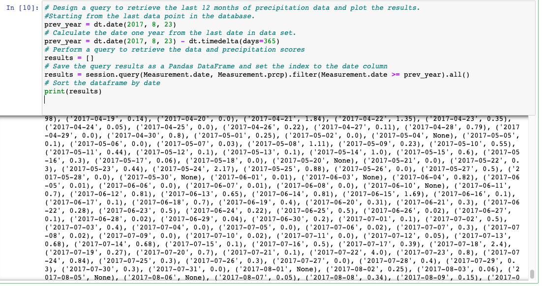
We'll design a query to retrieve the last 12 months of precipitation data and plot the results. Starting from the last data point in the database.
We have the last 12 months of precipitation data already loaded into the SQLite database. In the weather database, we'll calculate the date one year from August 23, 2017. We'll be creating a variable called
prev_yearand using the datetime dependency that we imported previously.
The datetime dependency has a function called dt.date(), which specifies the date in the following format: year, month, day.
Add the most recent date, August 23, 2017: prev_year = dt.date(2017, 8, 23)
Calculate the date one year back, adding the dt.timedelta() function to the code: prev_year = dt.date(2017, 8, 23) - dt.timedelta(days=365)
Retrieve the precipitation score - the amount of precipitation that was recorded.
Create a variable to store the results of the query: results = \[]
Add the session that we created earlier so that we can query our database:
For this we'll use the session.query() function (begin all of queries in SQLAlchemy).
The session.query() function for this query will take two parameters. We will reference the Measurement table using Measurement.date and Measurement.prcp.
results = session.query(Measurement.date, Measurement.prcp)To filter out all of the data that is older than a year from the last record date, We'll use the filter() function:
results = session.query(Measurement.date, Measurement.prcp).filter(Measurement.date >= prev_year)We'll also add a function that extracts all of the results from our query and put them in a list. We'll add .all() to the end of the existing query:
results = session.query(Measurement.date, Measurement.prcp).filter(Measurement.date >= prev_year).all()Run the final code:
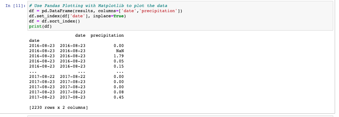
Save and load the query results into a Pandas DataFrame and set the index to the date column.
We have our weather results saved in a variable. In order to access it in the future, we'll save it to a Python Pandas DataFrame. We'll start by creating a DataFrame variable, df, which we can use to save our query results.
In order to save our results as a DataFrame, we need to provide our results variable as one parameter and specify the column names as our second parameter. To do this, we'll add the following line to our code:
df = pd.DataFrame(results, columns=['date','precipitation'])Use the set_index() Function
We want the index column to be the date column. We're also going to write over our original DataFrame. We can use the variable inplace to specify whether or not we want to create a new DataFrame. By setting inplace=True, we're saying that we do not want to create a new DataFrame with the modified specifications.
df.set_index(df['date'], inplace=True)Because we are using the date as the index, the DataFrame has two date columns, which is confusing. So we'll print the DataFrame without the index so we can see just the date and precipitation.
For this, we'll convert the DataFrame to strings, and then set our index to "False.":
print(df.to_string(index=False))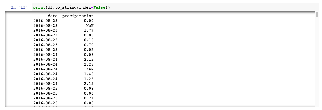
Sort the DataFrame values by date
To understand trends in the data we need to sort them. We're going to sort the values by date using the sort_index() function. Since we set our index to the date column previously, we can use our new index to sort our results.
df = df.sort_index()Final code:
Plot the Data
We'll plot the results using the DataFrame `plot` method:
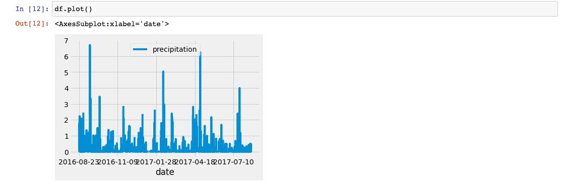
Along the x-axis are the dates from our dataset, and the y-axis is the total amount of precipitation for each day.
We can observe based on this plot that some months have higher amounts of precipitation than others.
Statistical analysis
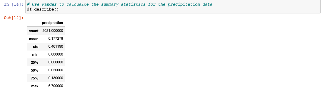
We'll use Pandas to print the summary statistics for the precipitation data.
In addition to the plot we'll determine the mean, standard deviation, minimum, and maximum.
Mean: the average, which you can find by adding up all the numbers in a dataset and dividing by the number of numbers.
Variance: how far a set of numbers is from the average.
Standard deviation: a measure of how spread out the numbers in a dataset are; the square root of the variance.
Minimum: the smallest number in a dataset.
Maximum: the largest number in a dataset. Percentiles: where the number is in relation to the rest of the set of data.
Count: the total number of numbers or items in a dataset.
We'll use the describe() function to calculate the mean, minimum, maximum, standard deviation, and percentiles.
Weather Station Analysis
Find the Number of Stations
We need to be sure that we have enough data collection stations for the information to be valid, so we need to determine how many stations are being used to collect the information.
- Design a query to calculate the total number of stations
We'll write a query to get the number of stations in our dataset. Begin with the starting point for the query: session.query()
Continuing with our query, we'll use func.count, which counts a given dataset. We can do this by referencing Station.station, which will give us the number of stations.
session.query(func.count(Station.station))Now we need to add the .all() function to the end of this query so that our results are returned as a list. Your final query should look like the following:
session.query(func.count(Station.station)).all()After run the query we get 9 station:

Design a query to find the most active stations
-- List the stations and observation counts in descending order.
-- Which station has the highest number of observations.
Next, we need to know how active the stations are as well (how much data has been collected from each station).
Begin with the function we use to start query in SQLAlchemy: session.query()
Next, we need to add a few parameters to our query. We'll list the stations and the counts, like this:
session.query(Measurement.station, func.count(Measurement.station))Now that we have our core query figured out, we'll add a few filters to narrow down the data to show only what we need.
We want to group the data by the station name, and then order by the count for each station in descending order. We're going to add group_by() first.
The whole code look like:
session.query(Measurement.station, func.count(Measurement.station)).\
    group_by(Measurement.station)
Now we'll add the order_by function which will order results in the order that we specify, in this case, descending order. Query results will be returned as a list.
After adding order_by(func.count(Measurement.station).desc()) , the code look like this:
session.query(Measurement.station, func.count(Measurement.station)).\
group_by(Measurement.station).order_by(func.count(Measurement.station).desc())
Now we need to add the .all() function here as well. This will return all of the results of our query.
The query will look like:
session.query(Measurement.station, func.count(Measurement.station)).\
group_by(Measurement.station).order_by(func.count(Measurement.station).desc()).all()
The results of the query:
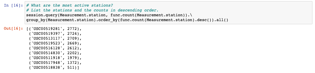
We can see which stations are the most and the least active.
Temperature Analysis (Low, High, and Average Temperatures)
We will calculate the minimum, maximum, and average temperatures with the following functions: func.min, func.max, and func.avg. Also we'll be filtering out everything but the most active station - USC00519281. Finally, add the .all() function to return our results as a list.
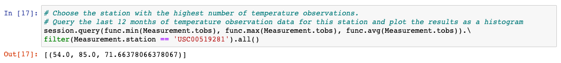
The results show that the low (minimum) temperature is 54 degrees, the high (maximum) temperature is 85 degrees, and the average temperature is approximately 72 degrees.
Plot the Highest Number of Observations
We need to create a plot that shows all of the temperatures in a given year for the station with the highest number of temperature observations.
- Create a Query for the Temperature Observations
To create a query, first select the column we are interested in. We want to pull Measurement.tobs in order to get our total observations count. EW will add this to the code:
session.query(Measurement.tobs)
Now filter out all the stations except the most active station with filter(Measurement.station == 'USC00519281'). The code will look like this:
results = session.query(Measurement.tobs).\
filter(Measurement.station == 'USC00519281')
We need to apply another filter to consider only the most recent year. For this we can reuse some of the code we have written previously. Then we'll add the .all() function to save our results as a list. Here's what your query should look like:
results = session.query(Measurement.tobs).\
filter(Measurement.station == 'USC00519281').\
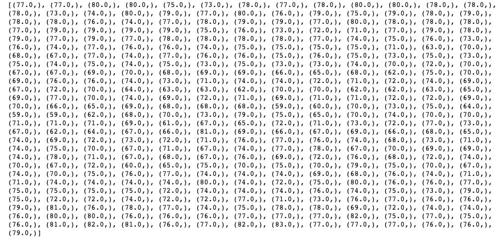
filter(Measurement.date >= prev_year).all()To run this code, we will need to add a print statement around it.
print(results)
The query results:
- Then we'll convert the temperature Observation results to a DataFrame to make the results easier to read, understand, and use.
When creating a DataFrame, our first parameter is our list, and the second parameter is the column(s) we want to put our data in. In this case, we want to put our temperature observations result list into a DataFrame.
To convert the results to a DataFrame, we will add the following to your code: df = pd.DataFrame(results, columns=\['tobs'])
- Plot the Temperature Observations
We'll be creating a histogram from the temperature observations. This will allow us to quickly count how many temperature observations we have.
We're going to divide our temperature observations into 12 different bins.
To create the histogram, we need to use the plot() function and the hist() function and add the number of bins as a parameter:
df.plot.hist(bins=12)
Using plt.tight_layout(), we can compress the x-axis labels so that they fit into the box holding our plot:
plt.tight_layout()
The whole code will be:
df = pd.DataFrame(results, columns=['tobs'])
df.plot.hist(bins=12)
plt.tight_layout()
and the results:
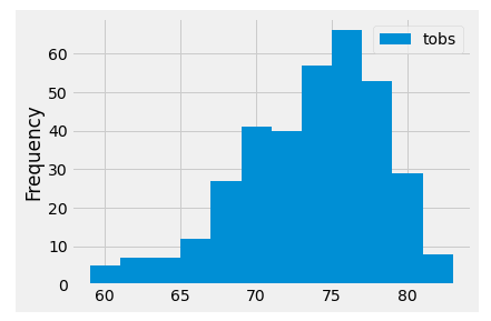
Looking at this plot, we can infer that a vast majority of the observations were over 67 degrees. If we count up the bins to the right of 67 degrees, we will get about 325 days where it was over 67 degrees when the temperature was observed.
Create a Climate App
We will design a Flask API based on the queries that we have just developed. We will use Flask to create our routes.
We're going to create five routes: Welcome, Precipitation, Stations, Monthly Temperature, and Statistics.
Set Up Flask and Create a Route
- Install Flask
pip install flask
pip install psycopg2-binary
- Create a Python file
Create a new Python file called app.py.
- Import the Flask dependency
from flask import Flask
- Create a new Flask app instance
app = Flask(\__name\_\_)
- Create Flask routes
@app.route('/')
Create a function called hello_world(). Whenever you make a route in Flask, you put the code you want in that specific route below @app.route().
@app.route('/')
def hello_world():
return 'Hello world'- Run a Flask app Use the command line to navigate to the folder where we've saved our python file. For Mac in terminal enter:
export FLASK_APP=app.py
then:
flask run
Run the brauser and go to localhost (the most common is localhost:5000).
Set Up the Database and Flask
Set Up the Flask Weather App
We'll put together a route for each segment of your analysis: Precipitation, Stations, Monthly Temperature, and Statistics.
First, we need to create a new Python file and import our dependencies to our code environment. Begin by creating a new Python file named app.py. This will be the file we use to create our Flask application.
Once the Python file is created, we'll get our dependencies imported: datetime, NumPy, and Pandas.
import datetime as dt
import numpy as np
import pandas as pd
Then we'll get the dependencies we need for SQLAlchemy, which will help to access our data in the SQLite database:
import sqlalchemy
from sqlalchemy.ext.automap import automap_base
from sqlalchemy.orm import Session
from sqlalchemy import create_engine, func
Finally, we'll add the code to import the dependencies that we need for Flask:
from flask import Flask, jsonifySet Up the Database
We'll set up our database engine for the Flask application, which allows us to access and query our SQLite database file:
engine = create_engine("sqlite:///hawaii.sqlite")
Then, reflect the database into our classes
Base = automap_base()
Then, reflect the tables:
Base.prepare(engine, reflect=True)
With the database reflected, we can save our references to each table. We'll create a variable for each of the classes so that we can reference them later:
Measurement = Base.classes.measurement
Station = Base.classes.station
Finally, create a session link from Python to our database with the following code:
session = Session(engine)
Then, we'll define the app for a Flask application. This will create a Flask application called "app.":
app = Flask(\__name\_\_)
Build Flask routes
Create the Welcome Route
We want our welcome route to be the root, which in our case is essentially the homepage.
All of our routes should go after the app = Flask(\__name\_\_) line of code.
We can define the welcome route using the code below:
@app.route("/")
Now our root, or welcome route, is set up. The next step is to add the routing information for each of the other routes. For this we'll create a function, and our return statement will have f-strings as a reference to all of the other routes.
First, we'll create a function welcome() with a return statement.
def welcome():
   return
Next, we'll add the precipitation, stations, tobs, and temp routes that we'll need into our return statement. We'll use f-strings to display them.
def welcome():
    return(
    '''
    Welcome to the Climate Analysis API!
    Available Routes:
    /api/v1.0/precipitation
    /api/v1.0/stations
    /api/v1.0/tobs
    /api/v1.0/temp/start/end
    ''')
Next, we'll split up the code we wrote for the temperature analysis, precipitation analysis, and station analysis, and apply it to the respective routes.
Create the Precipitation Route
The next route we'll build is for the precipitation analysis. This route will occur separately from the welcome route.
To create the route, we'll add the following code:
@app.route("/api/v1.0/precipitation")
Next, we will create the precipitation() function.
def precipitation():
    return
We'll add the line of code that calculates the date one year ago from the most recent date in the database and write a query to get the date and precipitation for the previous year:
def precipitation():
prev_year = dt.date(2017, 8, 23) - dt.timedelta(days=365)
precipitation = session.query(Measurement.date, Measurement.prcp).\
filter(Measurement.date >= prev_year).all()
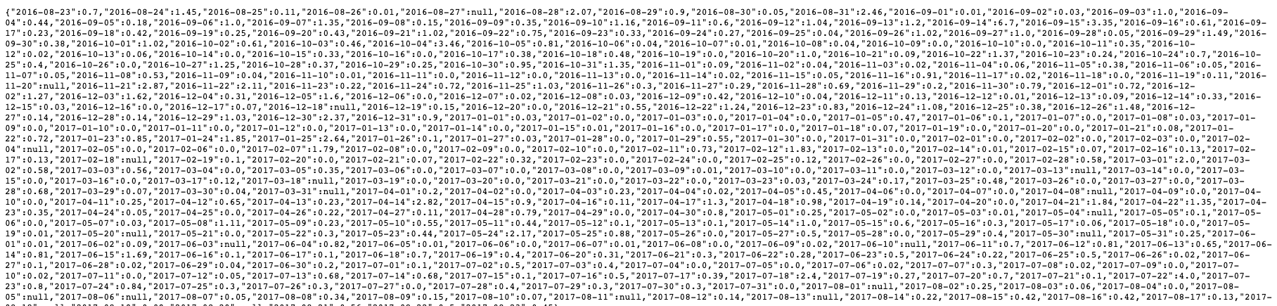
returnFinally, we'll create a dictionary with the date as the key and the precipitation as the value. To do this, we will "jsonify" our dictionary. jsonify() is a function that converts the dictionary to a JSON file.
We'll use jsonify() to format our results into a JSON structured file. When we run this code, we'll see what the JSON file structure looks like.
def precipitation():
   prev_year = dt.date(2017, 8, 23) - dt.timedelta(days=365)
   precipitation = session.query(Measurement.date, Measurement.prcp).\
    filter(Measurement.date >= prev_year).all()
   precip = {date: prcp for date, prcp in precipitation}
   return jsonify(precip)
After run our code we can see the output (http://127.0.0.1:5000/api/v1.0/precipitation):
Create the Stations Route
For this route we'll simply return a list of all the stations.
Begin by defining the route and route name. This code should occur outside of the previous route and have no indentation. We'll add this route to our code:
@app.route("/api/v1.0/stations")
With our route defined, we'll create a new function called stations():
def stations():
    return
Now we need to create a query that will allow us to get all of the stations in our database. Let's add that functionality to our code:
def stations():
    results = session.query(Station.station).all()
    return
We want to start by unraveling our results into a one-dimensional array. To do this, we want to use the function np.ravel(), with results as our parameter.
Next, we will convert our unraveled results into a list. To convert the results to a list, we will need to use the list function, which is list(), and then convert that array into a list. Then we'll jsonify the list and return it as JSON:
def stations():
    results = session.query(Station.station).all()
    stations = list(np.ravel(results))
    return jsonify(stations=stations)
After run our code we can see the output (http://127.0.0.1:5000/api/v1.0/stations):

Create the Temperature Observations Route
For this route, the goal is to return the temperature observations for the previous year. As with the previous routes, we'll begin by defining the route with this code:
@app.route("/api/v1.0/tobs")
Next, create a function called temp_monthly() by adding the following code:
def temp_monthly():
    return
Now, calculate the date one year ago from the last date in the database. (This is the same date as the one we calculated previously):
def temp_monthly():
    prev_year = dt.date(2017, 8, 23) - dt.timedelta(days=365)
    return
The next step is to query the primary station for all the temperature observations from the previous year. Here's what the code should look like with the query statement added:
def temp_monthly():
    prev_year = dt.date(2017, 8, 23) - dt.timedelta(days=365)
    results = session.query(Measurement.tobs).\
        filter(Measurement.station == 'USC00519281').\
        filter(Measurement.date >= prev_year).all()
    return
Finally, as before, unravel the results into a one-dimensional array and convert that array into a list. Then jsonify the list and return our results, like this:
def temp_monthly():
    prev_year = dt.date(2017, 8, 23) - dt.timedelta(days=365)
    results = session.query(Measurement.tobs).\
      filter(Measurement.station == 'USC00519281').\
      filter(Measurement.date >= prev_year).all()
    temps = list(np.ravel(results))
As we did earlier, we want to jsonify our temps list, and then return it. Add the return statement to the end of your code so that the route looks like this:
def temp_monthly():
    prev_year = dt.date(2017, 8, 23) - dt.timedelta(days=365)
    results = session.query(Measurement.tobs).\
      filter(Measurement.station == 'USC00519281').\
      filter(Measurement.date >= prev_year).all()
    temps = list(np.ravel(results))
    return jsonify(temps=temps)
After run our code we can see the output (http://127.0.0.1:5000/api/v1.0/tobs):

Create a Route for the Statistics Analysis
Our last route will be to report on the minimum, average, and maximum temperatures. However, this route is different from the previous ones in that we will have to provide both a starting and ending date.
@app.route("/api/v1.0/temp/<start>")
@app.route("/api/v1.0/temp/<start>/<end>")
Next, we'll create a function called stats() to put our code in:
def stats():
     return
We need to add parameters to our stats()function: a start parameter and an end parameter. For now, set them both to None.
def stats(start=None, end=None):
     return
With the function declared, we can now create a query to select the minimum, average, and maximum temperatures from our SQLite database. We'll start by just creating a list called sel, with the following code:
def stats(start=None, end=None):
    sel = [func.min(Measurement.tobs), func.avg(Measurement.tobs), func.max(Measurement.tobs)]
Since we need to determine the starting and ending date, add an if-not statement to our code. This will help us accomplish a few things. We'll need to query our database using the list that we just made. Then, we'll unravel the results into a one-dimensional array and convert them to a list. Finally, we will jsonify our results and return them.
In the following code, take note of the asterisk in the query next to the sel list. Here the asterisk is used to indicate there will be multiple results for our query: minimum, average, and maximum temperatures.
def stats(start=None, end=None):
    sel = [func.min(Measurement.tobs), func.avg(Measurement.tobs), func.max(Measurement.tobs)]

    if not end:
        results = session.query(*sel).\
            filter(Measurement.date >= start).all()
        temps = list(np.ravel(results))
        return jsonify(temps=temps)
Now we need to calculate the temperature minimum, average, and maximum with the start and end dates. We'll use the sel list, which is simply the data points we need to collect. We'll create our next query, which will get our statistics data.
def stats(start=None, end=None):
    sel = [func.min(Measurement.tobs), func.avg(Measurement.tobs), func.max(Measurement.tobs)]

    if not end:
        results = session.query(*sel).\
            filter(Measurement.date >= start).all()
        temps = list(np.ravel(results))
        return jsonify(temps)

    results = session.query(*sel).\
        filter(Measurement.date >= start).\
        filter(Measurement.date <= end).all()
    temps = list(np.ravel(results))
    return jsonify(temps)
After run our code we can see the output (http://127.0.0.1:5000/api/v1.0/temp/start/end route):
\[null,null,null]
This code tells us that we have not specified a start and end date for our range. Fix this by entering any date in the dataset as a start and end date. The code will output the minimum, maximum, and average temperatures. For example, let's say we want to find the minimum, maximum, and average temperatures for June 2017. We would add the following path to the address in our web browser:
/api/v1.0/temp/2017-06-01/2017-06-30When we run the code, it will return the following result:
["temps":[71.0,77.21989528795811,83.0]]